
As carbon dioxide levels in the earth’s atmosphere reach record levels, NASA presents some of the lesser known facts you need to know about greenhouse gases
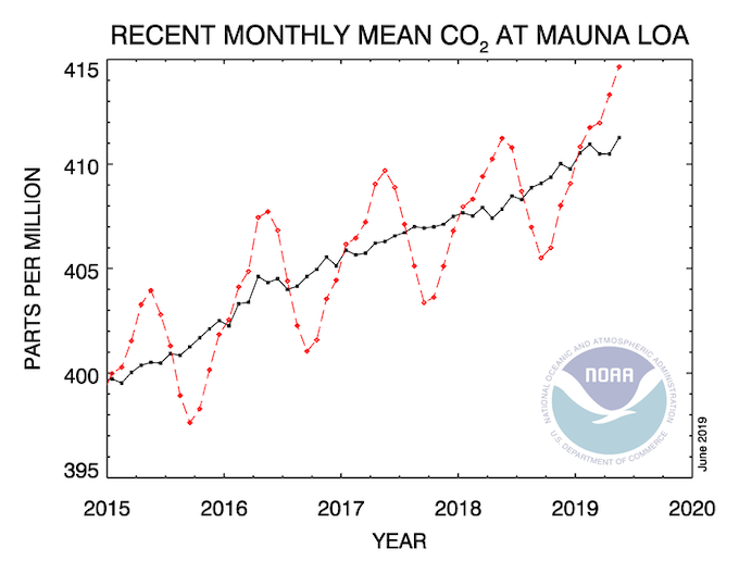
In May 2019, when atmospheric carbon dioxide reached its yearly peak, it set a record. The May average concentration of the greenhouse gas was 414.7 parts per million (ppm), as observed at NOAA’s Mauna Loa Atmospheric Baseline Observatory in Hawaii. That was the highest seasonal peak in 61 years, and the seventh consecutive year with a steep increase, according to NOAA and the Scripps Institution of Oceanography.
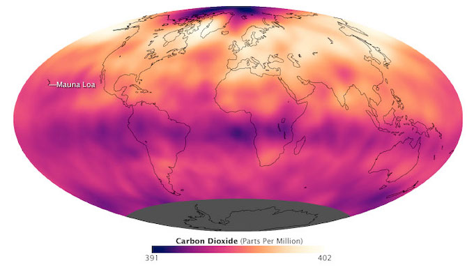
The Mauna Loa Observatory has been measuring carbon dioxide since 1958. The remote location (high on a volcano) and scarce vegetation make it a good place to monitor carbon dioxide because it does not have much interference from local sources of the gas. (There are occasional volcanic emissions, but scientists can easily monitor and filter them out.) Mauna Loa is part of a globally distributed network of air sampling sites that measure how much carbon dioxide is in the atmosphere.
The broad consensus among climate scientists is that increasing concentrations of carbon dioxide in the atmosphere are causing temperatures to warm, sea levels to rise, oceans to grow more acidic, and rainstorms, droughts, floods and fires to become more severe. Here are six less widely known but interesting things to know about carbon dioxide.
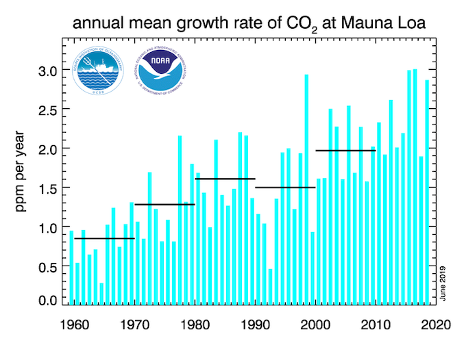
Accelerated increase
For decades, carbon dioxide concentrations have been increasing every year. In the 1960s, Mauna Loa saw annual increases around 0.8 ppm per year. By the 1980s and 1990s, the growth rate was up to 1.5 ppm year. Now it is above 2 ppm per year. There is “abundant and conclusive evidence” that the acceleration is caused by increased emissions, according to Pieter Tans, senior scientist with NOAA’s Global Monitoring Division.
To understand carbon dioxide variations prior to 1958, scientists rely on ice cores. Researchers have drilled deep into icepack in Antarctica and Greenland and taken samples of ice that are thousands of years old. That old ice contains trapped air bubbles that make it possible for scientists to reconstruct past carbon dioxide levels.
Uneven distribution
Satellite observations show carbon dioxide in the air can be somewhat patchy, with high concentrations in some places and lower concentrations in others. For instance, the map below shows carbon dioxide levels for May 2013 in the mid-troposphere, the part of the atmosphere where most weather occurs. At the time there was more carbon dioxide in the northern hemisphere because crops, grasses, and trees hadn’t greened up yet and absorbed some of the gas. The transport and distribution of CO2 throughout the atmosphere is controlled by the jet stream, large weather systems, and other large-scale atmospheric circulations. This patchiness has raised interesting questions about how carbon dioxide is transported from one part of the atmosphere to another—both horizontally and vertically.
Patchy mixing
In this animation from NASA’s Scientific Visualization Studio, big plumes of carbon dioxide stream from cities in North America, Asia, and Europe. They also rise from areas with active crop fires or wildfires. Yet these plumes quickly get mixed as they rise and encounter high-altitude winds. In the visualization, reds and yellows show regions of higher than average CO2, while blues show regions lower than average. The pulsing of the data is caused by the day/night cycle of plant photosynthesis at the ground. This view highlights carbon dioxide emissions from crop fires in South America and Africa. The carbon dioxide can be transported over long distances, but notice how mountains can block the flow of the gas.
You’ll notice that there is a distinct sawtooth pattern in charts that show how carbon dioxide is changing over time. There are peaks and dips in carbon dioxide caused by seasonal changes in vegetation. Plants, trees, and crops absorb carbon dioxide, so seasons with more vegetation have lower levels of the gas. Carbon dioxide concentrations typically peak in April and May because decomposing leaves in forests in the Northern Hemisphere (particularly Canada and Russia) have been adding carbon dioxide to the air all winter, while new leaves have not yet sprouted and absorbed much of the gas. In the chart and maps below, the ebb and flow of the carbon cycle is visible by comparing the monthly changes in carbon dioxide with the globe’s net primary productivity, a measure of how much carbon dioxide vegetation consume during photosynthesis minus the amount they release during respiration. Notice that carbon dioxide dips in Northern Hemisphere summer.
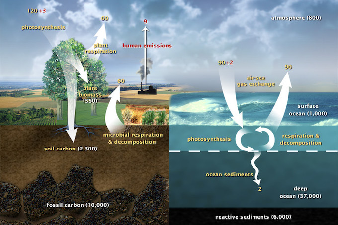
Not just the atmosphere
Most of Earth’s carbon—about 65,500 billion metric tons—is stored in rocks. The rest resides in the ocean, atmosphere, plants, soil, and fossil fuels. Carbon flows between each reservoir in the carbon cycle, which has slow and fast components. Any change in the cycle that shifts carbon out of one reservoir puts more carbon into other reservoirs. Any changes that put more carbon gases into the atmosphere result in warmer air temperatures. That’s why burning fossil fuels or wildfires are not the only factors determining what happens with atmospheric carbon dioxide. Things like the activity of phytoplankton, the health of the world’s forests, and the ways we change the landscapes through farming or building can play critical roles as well.
This article was first posted on Indian climate dialogue.